| Autor: | Pauli Virtanen |
|---|
Numpy se encuentra en la base del montón de herramientas científicas de Python. Su propósito es simple: implementar operaciones eficientes sobre muchos items en un bloque de memoria. Entender detalladamente como funciona sirve de ayuda para poder hacer un uso más eficiente de su flexibilidad, usando útiles atajos y creando nuevo trabajo basado en él.
Este tutorial pretende cubrir:
Preerequisitos
En esta sección numpy será importado de la siguiente forma
>>> import numpy as np
Contenido
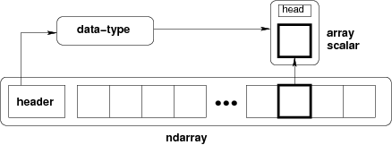
ndarray =
bloque de memoria + esquema de indexación + descriptor del tipo de dato
- Dato bruto (raw data)
- Cómo localizar un elemento
- Cómo interpretar un elemento
typedef struct PyArrayObject {
        PyObject_HEAD

        /* Block of memory */
        char *data;

        /* Data type descriptor */
        PyArray_Descr *descr;

        /* Indexing scheme */
        int nd;
        npy_intp *dimensions;
        npy_intp *strides;

        /* Other stuff */
        PyObject *base;
        int flags;
        PyObject *weakreflist;
} PyArrayObject;
>>> x = np.array([1, 2, 3, 4], dtype=np.int32)
>>> x.data
<read-write buffer for ..., size 16, offset 0 at ...>
>>> str(x.data)
'\x01\x00\x00\x00\x02\x00\x00\x00\x03\x00\x00\x00\x04\x00\x00\x00'
Dirección en memoria de los datos:
>>> x.__array_interface__['data'][0]
64803824
Recordatorio: dos ndarrays deben compartir la misma memoria:
>>> x = np.array([1, 2, 3, 4])
>>> y = x[:-1]
>>> x[0] = 9
>>> y
array([9, 2, 3])
La memoria no tiene que pertenecer a un ndarray:
>>> x = '1234'
>>> y = np.frombuffer(x, dtype=np.int8)
>>> y.data
<read-only buffer for ..., size 4, offset 0 at ...>
>>> y.base is x
True

>>> y.flags
  C_CONTIGUOUS : True
  F_CONTIGUOUS : True
  OWNDATA : False
  WRITEABLE : False
  ALIGNED : True
  UPDATEIFCOPY : False
Los flags owndata y writeable indican el estátus de la memoria.
dtype describe un único item en el array:
| type | scalar type de los datos, puede ser uno de: int8, int16, float64, et al. (tamaño fijo) str, unicode, void (tamaño flexible) |
| itemsize | tamaño del bloque de datos |
| byteorder | byte order: big-endian > / little-endian < / not applicable | |
| fields | sub-dtypes, si es un tipo de datos estructurados |
| shape | forma del array, si es un sub-array |
>>> np.dtype(int).type
<type 'numpy.int64'>
>>> np.dtype(int).itemsize
8
>>> np.dtype(int).byteorder
'='
El cabecero del fichero .wav:
| chunk_id | "RIFF" |
| chunk_size | 4-byte unsigned little-endian integer |
| format | "WAVE" |
| fmt_id | "fmt " |
| fmt_size | 4-byte unsigned little-endian integer |
| audio_fmt | 2-byte unsigned little-endian integer |
| num_channels | 2-byte unsigned little-endian integer |
| sample_rate | 4-byte unsigned little-endian integer |
| byte_rate | 4-byte unsigned little-endian integer |
| block_align | 2-byte unsigned little-endian integer |
| bits_per_sample | 2-byte unsigned little-endian integer |
| data_id | "data" |
| data_size | 4-byte unsigned little-endian integer |
El cabecero del fichero .wav como un tipo de datos estructurados Numpy:
>>> wav_header_dtype = np.dtype([
...     ("chunk_id", (str, 4)),   # flexible-sized scalar type, item size 4
...     ("chunk_size", "<u4"),    # little-endian unsigned 32-bit integer
...     ("format", "S4"),         # 4-byte string
...     ("fmt_id", "S4"),
...     ("fmt_size", "<u4"),
...     ("audio_fmt", "<u2"),     #
...     ("num_channels", "<u2"),  # .. more of the same ...
...     ("sample_rate", "<u4"),   #
...     ("byte_rate", "<u4"),
...     ("block_align", "<u2"),
...     ("bits_per_sample", "<u2"),
...     ("data_id", ("S1", (2, 2))), # sub-array, just for fun!
...     ("data_size", "u4"),
...     #
...     # the sound data itself cannot be represented here:
...     # it does not have a fixed size
...    ])
Ver también
wavreader.py
>>> wav_header_dtype['format']
dtype('|S4')
>>> wav_header_dtype.fields
<dictproxy object at ...>
>>> wav_header_dtype.fields['format']
(dtype('|S4'), 8)
Ejercicio
Mini-ejercicio, hacer un dtype “disperso” usando offsets y solo algunos de los campos:
>>> wav_header_dtype = np.dtype(dict(
...   names=['format', 'sample_rate', 'data_id'],
...   offsets=[offset_1, offset_2, offset_3], # counted from start of structure in bytes
...   formats=list of dtypes for each of the fields,
... ))
y usar eso para leer la tasa de muestreo (sample rate) y data_id (como sub-array).
>>> f = open('data/test.wav', 'r')
>>> wav_header = np.fromfile(f, dtype=wav_header_dtype, count=1)
>>> f.close()
>>> print(wav_header)
[ ('RIFF', 17402L, 'WAVE', 'fmt ', 16L, 1, 1, 16000L, 32000L, 2, 16, [['d', 'a'], ['t', 'a']], 17366L)]
>>> wav_header['sample_rate']
array([16000], dtype=uint32)
Vamos a intentar acceder al sub-array:
>>> wav_header['data_id']
array([[['d', 'a'],
        ['t', 'a']]],
      dtype='|S1')
>>> wav_header.shape
(1,)
>>> wav_header['data_id'].shape
(1, 2, 2)
¡Cuando accedemos a sub-arrays las dimensiones se añaden al final!
Nota
Existen módulos como wavfile, audiolab, etc. para leer datos de sonido...
casting (o transformación de tipo)
- al asignar
- en la construcción de arrays
- en aritmética
- etc.
- y manualmente: .astype(dtype)
re-interpretación de dato
- manualmente: .view(dtype)
Casting en aritmética, resumiendo:
Casting en copias generales de datos:
>>> x = np.array([1, 2, 3, 4], dtype=np.float)
>>> x
array([ 1.,  2.,  3.,  4.])
>>> y = x.astype(np.int8)
>>> y
array([1, 2, 3, 4], dtype=int8)
>>> y + 1
array([2, 3, 4, 5], dtype=int8)
>>> y + 256
array([1, 2, 3, 4], dtype=int8)
>>> y + 256.0
array([ 257.,  258.,  259.,  260.])
>>> y + np.array([256], dtype=np.int32)
array([257, 258, 259, 260], dtype=int32)
Casting en setitem: dtype del array no cambia al asignar al item:
>>> y[:] = y + 1.5
>>> y
array([2, 3, 4, 5], dtype=int8)
Nota
Para conocer las reglas exactas: ver la documentación: http://docs.scipy.org/doc/numpy/reference/ufuncs.html#casting-rules
Bloques de datos en memoria (4 bytes)
| 0x01 | || | 0x02 | || | 0x03 | || | 0x04 |
¿Cómo cambiar de uno a otro?
Cambiando el dtype:
>>> x = np.array([1, 2, 3, 4], dtype=np.uint8)
>>> x.dtype = "<i2"
>>> x
array([ 513, 1027], dtype=int16)
>>> 0x0201, 0x0403
(513, 1027)
0x01 0x02 || 0x03 0x04 Nota
little-endian: el byte menos significativo se encuentra a la izquierda en memoria
Creando una nueva vista:
>>> y = x.view("<i4")
>>> y
array([67305985], dtype=int32)
>>> 0x04030201
67305985
0x01 0x02 0x03 0x04
Nota
.view() crea vistas, no copia (o altera) el bloque de memoria
solo cambia el dtype (y ajusta la forma del array):
>>> x[1] = 5
>>> y
array([328193], dtype=int32)
>>> y.base is x
True
Mini-ejercicio: re-interpretación de datos
Ver también
view-colors.py
Tenemos datos RGBA en un array:
>>> x = np.zeros((10, 10, 4), dtype=np.int8)
>>> x[:, :, 0] = 1
>>> x[:, :, 1] = 2
>>> x[:, :, 2] = 3
>>> x[:, :, 3] = 4
donde la tercera dimensión indica cada uno de los canales R, B, and G y alpha.
¿Cómo hacer un array estructurado (10, 10) con los field names ‘r’, ‘g’, ‘b’, ‘a’ sin crear una copia de los datos?
>>> y = ...

>>> assert (y['r'] == 1).all()
>>> assert (y['g'] == 2).all()
>>> assert (y['b'] == 3).all()
>>> assert (y['a'] == 4).all()
Solución
Advertencia
Otro array tomando, exactamente, 4 bytes de memoria:
>>> y = np.array([[1, 3], [2, 4]], dtype=np.uint8).transpose()
>>> x = y.copy()
>>> x
array([[1, 2],
       [3, 4]], dtype=uint8)
>>> y
array([[1, 2],
       [3, 4]], dtype=uint8)
>>> x.view(np.int16)
array([[ 513],
       [1027]], dtype=int16)
>>> 0x0201, 0x0403
(513, 1027)
>>> y.view(np.int16)
array([[ 769, 1026]], dtype=int16)
>>> 0x0301, 0x0402
(769, 1026)
La pregunta
>>> x = np.array([[1, 2, 3],
...              [4, 5, 6],
...              [7, 8, 9]], dtype=np.int8)
>>> str(x.data)
'\x01\x02\x03\x04\x05\x06\x07\x08\t'
¿En qué byte en x.data commienza el item x[1,2]?
La respuesta (en Numpy)
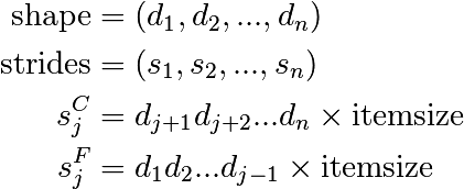
- strides (o pasos): El número de bytes a saltar para encontrar el siguiente elemento
- 1 stride por dimensión
>>> x.strides
(3, 1)
>>> byte_offset = 3*1 + 1*2   # to find x[1,2]
>>> x.data[byte_offset]
'\x06'
>>> x[1, 2]
6
- simple, flexible
>>> x = np.array([[1, 2, 3],
...               [4, 5, 6],
...               [7, 8, 9]], dtype=np.int16, order='C')
>>> x.strides
(6, 2)
>>> str(x.data)
'\x01\x00\x02\x00\x03\x00\x04\x00\x05\x00\x06\x00\x07\x00\x08\x00\t\x00'
>>> y = np.array(x, order='F')
>>> y.strides
(2, 6)
>>> str(y.data)
'\x01\x00\x04\x00\x07\x00\x02\x00\x05\x00\x08\x00\x03\x00\x06\x00\t\x00'
De forma similar para dimensiones mayores:
Nota
Ahora podemos entender el comportamiento de .view():
>>> y = np.array([[1, 3], [2, 4]], dtype=np.uint8).transpose()
>>> x = y.copy()
La transposición no afecta al layout de memoria de los datos, solo a los strides
>>> x.strides
(2, 1)
>>> y.strides
(1, 2)
>>> str(x.data)
'\x01\x02\x03\x04'
>>> str(y.data)
'\x01\x03\x02\x04'
Nota
NdT: Slicing, traducido literalmente, significa rebanada, rodaja. Con este término nos referimos a tomar una porción/rodaja/rebanada de los datos, es decir, usar un subconjunto de los datos disponibles en el array
>>> x = np.array([1, 2, 3, 4, 5, 6], dtype=np.int32)
>>> y = x[::-1]
>>> y
array([6, 5, 4, 3, 2, 1], dtype=int32)
>>> y.strides
(-4,)
>>> y = x[2:]
>>> y.__array_interface__['data'][0] - x.__array_interface__['data'][0]
8
>>> x = np.zeros((10, 10, 10), dtype=np.float)
>>> x.strides
(800, 80, 8)
>>> x[::2,::3,::4].strides
(1600, 240, 32)
Stride manipulation
>>> from numpy.lib.stride_tricks import as_strided
>>> help(as_strided)
as_strided(x, shape=None, strides=None)
   Make an ndarray from the given array with the given shape and strides
Advertencia
as_strided does not check that you stay inside the memory block bounds...
>>> x = np.array([1, 2, 3, 4], dtype=np.int16)
>>> as_strided(x, strides=(2*2, ), shape=(2, ))
array([1, 3], dtype=int16)
>>> x[::2]
array([1, 3], dtype=int16)
Ver también
stride-fakedims.py
Exercise
array([1, 2, 3, 4], dtype=np.int8)

-> array([[1, 2, 3, 4],
          [1, 2, 3, 4],
          [1, 2, 3, 4]], dtype=np.int8)
using only as_strided.:
Hint: byte_offset = stride[0]*index[0] + stride[1]*index[1] + ...
Spoiler
>>> x = np.array([1, 2, 3, 4], dtype=np.int16)
>>> x2 = as_strided(x, strides=(0, 1*2), shape=(3, 4))
>>> x2
array([[1, 2, 3, 4],
       [1, 2, 3, 4],
       [1, 2, 3, 4]], dtype=int16)
>>> y = np.array([5, 6, 7], dtype=np.int16)
>>> y2 = as_strided(y, strides=(1*2, 0), shape=(3, 4))
>>> y2
array([[5, 5, 5, 5],
       [6, 6, 6, 6],
       [7, 7, 7, 7]], dtype=int16)
>>> x2 * y2
array([[ 5, 10, 15, 20],
       [ 6, 12, 18, 24],
       [ 7, 14, 21, 28]], dtype=int16)
... seems somehow familiar ...
>>> x = np.array([1, 2, 3, 4], dtype=np.int16)
>>> y = np.array([5, 6, 7], dtype=np.int16)
>>> x[np.newaxis,:] * y[:,np.newaxis]
array([[ 5, 10, 15, 20],
       [ 6, 12, 18, 24],
       [ 7, 14, 21, 28]], dtype=int16)
Ver también
stride-diagonals.py
Challenge
Pick diagonal entries of the matrix: (assume C memory order):
>>> x = np.array([[1, 2, 3],
...               [4, 5, 6],
...               [7, 8, 9]], dtype=np.int32)

>>> x_diag = as_strided(x, shape=(3,), strides=(???,))
Pick the first super-diagonal entries [2, 6].
And the sub-diagonals?
- (Hint to the last two: slicing first moves the point where striding
- starts from.)
Solution
Ver también
stride-diagonals.py
Challenge
Compute the tensor trace:
>>> x = np.arange(5*5*5*5).reshape(5,5,5,5)
>>> s = 0
>>> for i in xrange(5):
...    for j in xrange(5):
...       s += x[j,i,j,i]
by striding, and using sum() on the result.
>>> y = as_strided(x, shape=(5, 5), strides=(TODO, TODO))
>>> s2 = ...
>>> assert s == s2
Solution
Memory layout can affect performance:
In [1]: x = np.zeros((20000,))

In [2]: y = np.zeros((20000*67,))[::67]

In [3]: x.shape, y.shape
((20000,), (20000,))

In [4]: %timeit x.sum()
100000 loops, best of 3: 0.180 ms per loop

In [5]: %timeit y.sum()
100000 loops, best of 3: 2.34 ms per loop

In [6]: x.strides, y.strides
((8,), (536,))
Smaller strides are faster?
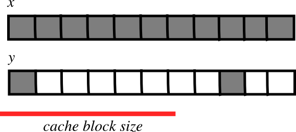
 fewer transfers needed faster
Ver también
numexpr is designed to mitigate cache effects in array computing.
Sometimes,
>>> a -= b
is not the same as
>>> a -= b.copy()
>>> x = np.array([[1, 2], [3, 4]])
>>> x -= x.transpose()
>>> x
array([[ 0, -1],
       [ 4,  0]])
>>> y = np.array([[1, 2], [3, 4]])
>>> y -= y.T.copy()
>>> y
array([[ 0, -1],
       [ 1,  0]])
Ufunc performs and elementwise operation on all elements of an array.
Examples:
np.add, np.subtract, scipy.special.*, ...
Automatically support: broadcasting, casting, ...
The author of an ufunc only has to supply the elementwise operation, Numpy takes care of the rest.
The elementwise operation needs to be implemented in C (or, e.g., Cython)
Provided by user
void ufunc_loop(void **args, int *dimensions, int *steps, void *data)
{
    /*
     * int8 output = elementwise_function(int8 input_1, int8 input_2)
     *
     * This function must compute the ufunc for many values at once,
     * in the way shown below.
     */
    char *input_1 = (char*)args[0];
    char *input_2 = (char*)args[1];
    char *output = (char*)args[2];
    int i;

    for (i = 0; i < dimensions[0]; ++i) {
        *output = elementwise_function(*input_1, *input_2);
        input_1 += steps[0];
        input_2 += steps[1];
        output += steps[2];
    }
}
The Numpy part, built by
char types[3]

types[0] = NPY_BYTE   /* type of first input arg */
types[1] = NPY_BYTE   /* type of second input arg */
types[2] = NPY_BYTE   /* type of third input arg */

PyObject *python_ufunc = PyUFunc_FromFuncAndData(
    ufunc_loop,
    NULL,
    types,
    1, /* ntypes */
    2, /* num_inputs */
    1, /* num_outputs */
    identity_element,
    name,
    docstring,
    unused)
ufunc_loop is of very generic form, and Numpy provides pre-made ones
| PyUfunc_f_f | float elementwise_func(float input_1) |
| PyUfunc_ff_f | float elementwise_func(float input_1, float input_2) |
| PyUfunc_d_d | double elementwise_func(double input_1) |
| PyUfunc_dd_d | double elementwise_func(double input_1, double input_2) |
| PyUfunc_D_D | elementwise_func(npy_cdouble *input, npy_cdouble* output) |
| PyUfunc_DD_D | elementwise_func(npy_cdouble *in1, npy_cdouble *in2, npy_cdouble* out) |
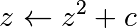
The Mandelbrot fractal is defined by the iteration
where  is a complex number. This iteration is
repeated – if
is a complex number. This iteration is
repeated – if  stays finite no matter how long the iteration
runs,
stays finite no matter how long the iteration
runs,  belongs to the Mandelbrot set.
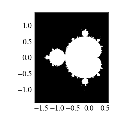
Make ufunc called mandel(z0, c) that computes:
z = z0
for k in range(iterations):
    z = z*z + c
say, 100 iterations or until z.real**2 + z.imag**2 > 1000. Use it to determine which c are in the Mandelbrot set.
Our function is a simple one, so make use of the PyUFunc_* helpers.
Write it in Cython
Ver también
mandel.pyx, mandelplot.py
Reminder: some pre-made Ufunc loops:
| PyUfunc_f_f | float elementwise_func(float input_1) |
| PyUfunc_ff_f | float elementwise_func(float input_1, float input_2) |
| PyUfunc_d_d | double elementwise_func(double input_1) |
| PyUfunc_dd_d | double elementwise_func(double input_1, double input_2) |
| PyUfunc_D_D | elementwise_func(complex_double *input, complex_double* output) |
| PyUfunc_DD_D | elementwise_func(complex_double *in1, complex_double *in2, complex_double* out) |
Type codes:
NPY_BOOL, NPY_BYTE, NPY_UBYTE, NPY_SHORT, NPY_USHORT, NPY_INT, NPY_UINT,
NPY_LONG, NPY_ULONG, NPY_LONGLONG, NPY_ULONGLONG, NPY_FLOAT, NPY_DOUBLE,
NPY_LONGDOUBLE, NPY_CFLOAT, NPY_CDOUBLE, NPY_CLONGDOUBLE, NPY_DATETIME,
NPY_TIMEDELTA, NPY_OBJECT, NPY_STRING, NPY_UNICODE, NPY_VOID
# The elementwise function
# ------------------------

cdef void mandel_single_point(double complex *z_in,
                              double complex *c_in,
                              double complex *z_out) nogil:
    #
    # The Mandelbrot iteration
    #

    #
    # Some points of note:
    #
    # - It's *NOT* allowed to call any Python functions here.
    #
    #   The Ufunc loop runs with the Python Global Interpreter Lock released.
    #   Hence, the ``nogil``.
    #
    # - And so all local variables must be declared with ``cdef``
    #
    # - Note also that this function receives *pointers* to the data;
    #   the "traditional" solution to passing complex variables around
    #

    cdef double complex z = z_in[0]
    cdef double complex c = c_in[0]
    cdef int k  # the integer we use in the for loop

    # Straightforward iteration

    for k in range(100):
        z = z*z + c
        if z.real**2 + z.imag**2 > 1000:
            break

    # Return the answer for this point
    z_out[0] = z


# Boilerplate Cython definitions
#
# You don't really need to read this part, it just pulls in
# stuff from the Numpy C headers.
# ----------------------------------------------------------

cdef extern from "numpy/arrayobject.h":
    void import_array()
    ctypedef int npy_intp
    cdef enum NPY_TYPES:
        NPY_CDOUBLE

cdef extern from "numpy/ufuncobject.h":
    void import_ufunc()
    ctypedef void (*PyUFuncGenericFunction)(char**, npy_intp*, npy_intp*, void*)
    object PyUFunc_FromFuncAndData(PyUFuncGenericFunction* func, void** data,
        char* types, int ntypes, int nin, int nout,
        int identity, char* name, char* doc, int c)

    void PyUFunc_DD_D(char**, npy_intp*, npy_intp*, void*)


# Required module initialization
# ------------------------------

import_array()
import_ufunc()


# The actual ufunc declaration
# ----------------------------

cdef PyUFuncGenericFunction loop_func[1]
cdef char input_output_types[3]
cdef void *elementwise_funcs[1]

loop_func[0] = PyUFunc_DD_D

input_output_types[0] = NPY_CDOUBLE
input_output_types[1] = NPY_CDOUBLE
input_output_types[2] = NPY_CDOUBLE

elementwise_funcs[0] = <void*>mandel_single_point

mandel = PyUFunc_FromFuncAndData(
    loop_func,
    elementwise_funcs,
    input_output_types,
    1, # number of supported input types
    2, # number of input args
    1, # number of output args
    0, # `identity` element, never mind this
    "mandel", # function name
    "mandel(z, c) -> computes iterated z*z + c", # docstring
    0 # unused
    )
import numpy as np
import mandel
x = np.linspace(-1.7, 0.6, 1000)
y = np.linspace(-1.4, 1.4, 1000)
c = x[None,:] + 1j*y[:,None]
z = mandel.mandel(c, c)

import matplotlib.pyplot as plt
plt.imshow(abs(z)**2 < 1000, extent=[-1.7, 0.6, -1.4, 1.4])
plt.gray()
plt.show()
Nota
Most of the boilerplate could be automated by these Cython modules:
Several accepted input types
E.g. supporting both single- and double-precision versions
cdef void mandel_single_point(double complex *z_in,
                              double complex *c_in,
                              double complex *z_out) nogil:
   ...

cdef void mandel_single_point_singleprec(float complex *z_in,
                                         float complex *c_in,
                                         float complex *z_out) nogil:
   ...

cdef PyUFuncGenericFunction loop_funcs[2]
cdef char input_output_types[3*2]
cdef void *elementwise_funcs[1*2]

loop_funcs[0] = PyUFunc_DD_D
input_output_types[0] = NPY_CDOUBLE
input_output_types[1] = NPY_CDOUBLE
input_output_types[2] = NPY_CDOUBLE
elementwise_funcs[0] = <void*>mandel_single_point

loop_funcs[1] = PyUFunc_FF_F
input_output_types[3] = NPY_CFLOAT
input_output_types[4] = NPY_CFLOAT
input_output_types[5] = NPY_CFLOAT
elementwise_funcs[1] = <void*>mandel_single_point_singleprec

mandel = PyUFunc_FromFuncAndData(
    loop_func,
    elementwise_funcs,
    input_output_types,
    2, # number of supported input types   <----------------
    2, # number of input args
    1, # number of output args
    0, # `identity` element, never mind this
    "mandel", # function name
    "mandel(z, c) -> computes iterated z*z + c", # docstring
    0 # unused
    )
ufunc
output = elementwise_function(input)
Both output and input can be a single array element only.
generalized ufunc
output and input can be arrays with a fixed number of dimensions
For example, matrix trace (sum of diag elements):
input shape = (n, n)
output shape = ()      i.e.  scalar

(n, n) -> ()
Matrix product:
input_1 shape = (m, n)
input_2 shape = (n, p)
output shape  = (m, p)

(m, n), (n, p) -> (m, p)
- This is called the “signature” of the generalized ufunc
- The dimensions on which the g-ufunc acts, are “core dimensions”
Status in Numpy
>>> import numpy.core.umath_tests as ut
>>> ut.matrix_multiply.signature
'(m,n),(n,p)->(m,p)'
>>> x = np.ones((10, 2, 4))
>>> y = np.ones((10, 4, 5))
>>> ut.matrix_multiply(x, y).shape
(10, 2, 5)
Generalized ufunc loop
Matrix multiplication (m,n),(n,p) -> (m,p)
void gufunc_loop(void **args, int *dimensions, int *steps, void *data)
{
    char *input_1 = (char*)args[0];  /* these are as previously */
    char *input_2 = (char*)args[1];
    char *output = (char*)args[2];

    int input_1_stride_m = steps[3];  /* strides for the core dimensions */
    int input_1_stride_n = steps[4];  /* are added after the non-core */
    int input_2_strides_n = steps[5]; /* steps */
    int input_2_strides_p = steps[6];
    int output_strides_n = steps[7];
    int output_strides_p = steps[8];

    int m = dimension[1]; /* core dimensions are added after */
    int n = dimension[2]; /* the main dimension; order as in */
    int p = dimension[3]; /* signature */

    int i;

    for (i = 0; i < dimensions[0]; ++i) {
        matmul_for_strided_matrices(input_1, input_2, output,
                                    strides for each array...);

        input_1 += steps[0];
        input_2 += steps[1];
        output += steps[2];
    }
}
Suppose you
Currently, 3 solutions:
Mini-exercise using PIL (Python Imaging Library):
Ver también
pilbuffer.py
>>> import Image
>>> data = np.zeros((200, 200, 4), dtype=np.int8)
>>> data[:, :] = [255, 0, 0, 255] # Red
>>> # In PIL, RGBA images consist of 32-bit integers whose bytes are [RR,GG,BB,AA]
>>> data = data.view(np.int32).squeeze()
>>> img = Image.frombuffer("RGBA", (200, 200), data)
>>> img.save('test.png')
Q:
Check what happens if data is now modified, and img saved again.
import numpy as np
import Image

# Let's make a sample image, RGBA format

x = np.zeros((200, 200, 4), dtype=np.int8)

x[:,:,0] = 254 # red
x[:,:,3] = 255 # opaque

data = x.view(np.int32) # Check that you understand why this is OK!

img = Image.frombuffer("RGBA", (200, 200), data)
img.save('test.png')

#
# Modify the original data, and save again.
#
# It turns out that PIL, which knows next to nothing about Numpy,
# happily shares the same data.
#

x[:,:,1] = 254
img.save('test2.png')


Ver también
Documentation: http://docs.scipy.org/doc/numpy/reference/arrays.interface.html
>>> x = np.array([[1, 2], [3, 4]])
>>> x.__array_interface__
{'data': (171694552, False),      # memory address of data, is readonly?
 'descr': [('', '<i4')],          # data type descriptor
 'typestr': '<i4',                # same, in another form
 'strides': None,                 # strides; or None if in C-order
 'shape': (2, 2),
 'version': 3,
}
>>> import Image
>>> img = Image.open('data/test.png')
>>> img.__array_interface__
{'data': ...,
 'shape': (200, 200, 4),
 'typestr': '|u1'}
>>> x = np.asarray(img)
>>> x.shape
(200, 200, 4)
>>> x.dtype
dtype('uint8')
Nota
A more C-friendly variant of the array interface is also defined.
>>> x = np.array(['a', '  bbb', '  ccc']).view(np.chararray)
>>> x.lstrip(' ')
chararray(['a', 'bbb', 'ccc'],
      dtype='|S5')
>>> x.upper()
chararray(['A', '  BBB', '  CCC'],
      dtype='|S5')
Nota
.view() has a second meaning: it can make an ndarray an instance of a specialized ndarray subclass
Masked arrays are arrays that may have missing or invalid entries.
For example, suppose we have an array where the fourth entry is invalid:
>>> x = np.array([1, 2, 3, -99, 5])
One way to describe this is to create a masked array:
>>> mx = np.ma.masked_array(x, mask=[0, 0, 0, 1, 0])
>>> mx
masked_array(data = [1 2 3 -- 5],
             mask = [False False False  True False],
       fill_value = 999999)
Masked mean ignores masked data:
>>> mx.mean()
2.75
>>> np.mean(mx)
2.75
Advertencia
Not all Numpy functions respect masks, for instance np.dot, so check the return types.
The masked_array returns a view to the original array:
>>> mx[1] = 9
>>> x
array([  1,   9,   3, -99,   5])
You can modify the mask by assigning:
>>> mx[1] = np.ma.masked
>>> mx
masked_array(data = [1 -- 3 -- 5],
             mask = [False  True False  True False],
       fill_value = 999999)
The mask is cleared on assignment:
>>> mx[1] = 9
>>> mx
masked_array(data = [1 9 3 -- 5],
             mask = [False False False  True False],
       fill_value = 999999)
The mask is also available directly:
>>> mx.mask
array([False, False, False,  True, False], dtype=bool)
The masked entries can be filled with a given value to get an usual array back:
>>> x2 = mx.filled(-1)
>>> x2
array([ 1,  9,  3, -1,  5])
The mask can also be cleared:
>>> mx.mask = np.ma.nomask
>>> mx
masked_array(data = [1 9 3 -99 5],
             mask = [False False False False False],
       fill_value = 999999)
The masked array package also contains domain-aware functions:
>>> np.ma.log(np.array([1, 2, -1, -2, 3, -5]))
masked_array(data = [0.0 0.69314718056 -- -- 1.09861228867 --],
             mask = [False False  True  True False  True],
       fill_value = 1e+20)
Nota
Streamlined and more seamless support for dealing with missing data in arrays is making its way into Numpy 1.7. Stay tuned!
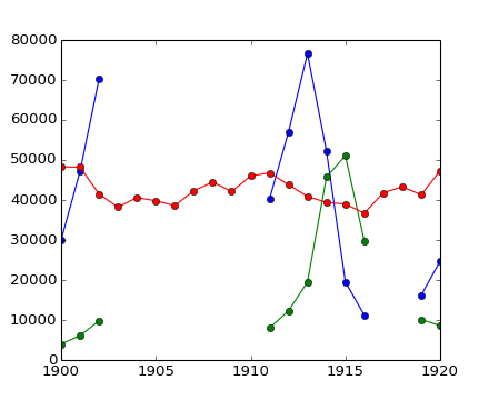
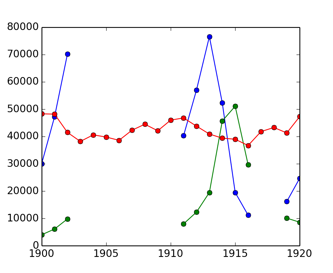
Example: Masked statistics
Canadian rangers were distracted when counting hares and lynxes in 1903-1910 and 1917-1918, and got the numbers are wrong. (Carrot farmers stayed alert, though.) Compute the mean populations over time, ignoring the invalid numbers.
>>> data = np.loadtxt('data/populations.txt')
>>> populations = np.ma.masked_array(data[:,1:])
>>> year = data[:, 0]

>>> bad_years = (((year >= 1903) & (year <= 1910))
...            | ((year >= 1917) & (year <= 1918)))
>>> # '&' means 'and' and '|' means 'or'
>>> populations[bad_years, 0] = np.ma.masked
>>> populations[bad_years, 1] = np.ma.masked

>>> populations.mean(axis=0)
masked_array(data = [40472.7272727 18627.2727273 42400.0],
             mask = [False False False],
       fill_value = 1e+20)

>>> populations.std(axis=0)
masked_array(data = [21087.656489 15625.7998142 3322.50622558],
             mask = [False False False],
       fill_value = 1e+20)
Note that Matplotlib knows about masked arrays:
>>> plt.plot(year, populations, 'o-')
[<matplotlib.lines.Line2D object at ...>, ...]
[source code, hires.png, pdf]
>>> arr = np.array([('a', 1), ('b', 2)], dtype=[('x', 'S1'), ('y', int)])
>>> arr2 = arr.view(np.recarray)
>>> arr2.x
chararray(['a', 'b'],
      dtype='|S1')
>>> arr2.y
array([1, 2])
>>> np.matrix([[1, 0], [0, 1]]) * np.matrix([[1, 2], [3, 4]])
matrix([[1, 2],
        [3, 4]])
Get this tutorial: http://www.euroscipy.org/talk/882
Title: numpy.random.permutations fails for non-integer arguments

I'm trying to generate random permutations, using numpy.random.permutations

When calling numpy.random.permutation with non-integer arguments
it fails with a cryptic error message::

    >>> np.random.permutation(12)
    array([ 6, 11,  4, 10,  2,  8,  1,  7,  9,  3,  0,  5])
    >>> np.random.permutation(12.)
    Traceback (most recent call last):
      File "<stdin>", line 1, in <module>
      File "mtrand.pyx", line 3311, in mtrand.RandomState.permutation
      File "mtrand.pyx", line 3254, in mtrand.RandomState.shuffle
    TypeError: len() of unsized object

This also happens with long arguments, and so
np.random.permutation(X.shape[0]) where X is an array fails on 64
bit windows (where shape is a tuple of longs).

It would be great if it could cast to integer or at least raise a
proper error for non-integer types.

I'm using Numpy 1.4.1, built from the official tarball, on Windows
64 with Visual studio 2008, on Python.org 64-bit Python.
What are you trying to do?
Small code snippet reproducing the bug (if possible)
Platform (Windows / Linux / OSX, 32/64 bits, x86/PPC, ...)
Version of Numpy/Scipy
>>> print np.__version__
2...
Check that the following is what you expect
>>> print np.__file__
/...
In case you have old/broken Numpy installations lying around.
If unsure, try to remove existing Numpy installations, and reinstall...
Documentation editor
Registration
Register an account
Subscribe to scipy-dev mailing list (subscribers-only)
Problem with mailing lists: you get mail
But: you can turn mail delivery off
“change your subscription options”, at the bottom of
Send a mail @ scipy-dev mailing list; ask for activation:
To: scipy-dev@scipy.org

Hi,

I'd like to edit Numpy/Scipy docstrings. My account is XXXXX

Cheers,
N. N.
- Check the style guide:
- http://docs.scipy.org/numpy/
- Don’t be intimidated; to fix a small thing, just fix it
- Edit
Edit sources and send patches (as for bugs)
Complain on the mailing list
Ask on mailing list, if unsure where it should go
Write a patch, add an enhancement ticket on the bug tracket
OR, create a Git branch implementing the feature + add enhancement ticket.
# Clone numpy repository
git clone --origin svn http://projects.scipy.org/git/numpy.git numpy
cd numpy

# Create a feature branch
git checkout -b name-of-my-feature-branch  svn/trunk

<edit stuff>

git commit -a
git remote add github git@github:YOURUSERNAME/YOURREPOSITORYNAME.git
git push github name-of-my-feature-branch
Bug fixes always welcome!
Documentation work
API docs: improvements to docstrings
User guide
Needs to be done eventually.
Want to think? Come up with a Table of Contents
Ask on communication channels:
