sparse matrix/eigenvalue problem solvers live in scipy.sparse.linalg
all solvers are accessible from:
>>> import scipy.sparse.linalg as spla
>>> spla.__all__
['LinearOperator', 'Tester', 'arpack', 'aslinearoperator', 'bicg',
'bicgstab', 'cg', 'cgs', 'csc_matrix', 'csr_matrix', 'dsolve',
'eigen', 'eigen_symmetric', 'factorized', 'gmres', 'interface',
'isolve', 'iterative', 'lgmres', 'linsolve', 'lobpcg', 'lsqr',
'minres', 'np', 'qmr', 'speigs', 'spilu', 'splu', 'spsolve', 'svd',
'test', 'umfpack', 'use_solver', 'utils', 'warnings']
import the whole module, and see its docstring:
>>> from scipy.sparse.linalg import dsolve
>>> help(dsolve)
both superlu and umfpack can be used (if the latter is installed) as follows:
prepare a linear system:
>>> import numpy as np
>>> from scipy import sparse
>>> mtx = sparse.spdiags([[1, 2, 3, 4, 5], [6, 5, 8, 9, 10]], [0, 1], 5, 5)
>>> mtx.todense()
matrix([[ 1,  5,  0,  0,  0],
        [ 0,  2,  8,  0,  0],
        [ 0,  0,  3,  9,  0],
        [ 0,  0,  0,  4, 10],
        [ 0,  0,  0,  0,  5]])
>>> rhs = np.array([1, 2, 3, 4, 5])
solve as single precision real:
>>> mtx1 = mtx.astype(np.float32)
>>> x = dsolve.spsolve(mtx1, rhs, use_umfpack=False)
>>> print x
[ 106.   -21.     5.5   -1.5    1. ]
>>> print "Error: ", mtx1 * x - rhs
Error:  [ 0.  0.  0.  0.  0.]
solve as double precision real:
>>> mtx2 = mtx.astype(np.float64)
>>> x = dsolve.spsolve(mtx2, rhs, use_umfpack=True)
>>> print x
[ 106.   -21.     5.5   -1.5    1. ]
>>> print "Error: ", mtx2 * x - rhs
Error:  [ 0.  0.  0.  0.  0.]
solve as single precision complex:
>>> mtx1 = mtx.astype(np.complex64)
>>> x = dsolve.spsolve(mtx1, rhs, use_umfpack=False)
>>> print x
[ 106.0+0.j  -21.0+0.j    5.5+0.j   -1.5+0.j    1.0+0.j]
>>> print "Error: ", mtx1 * x - rhs
Error:  [ 0.+0.j  0.+0.j  0.+0.j  0.+0.j  0.+0.j]
solve as double precision complex:
>>> mtx2 = mtx.astype(np.complex128)
>>> x = dsolve.spsolve(mtx2, rhs, use_umfpack=True)
>>> print x
[ 106.0+0.j  -21.0+0.j    5.5+0.j   -1.5+0.j    1.0+0.j]
>>> print "Error: ", mtx2 * x - rhs
Error:  [ 0.+0.j  0.+0.j  0.+0.j  0.+0.j  0.+0.j]
"""
Construct a 1000x1000 lil_matrix and add some values to it, convert it
to CSR format and solve A x = b for x:and solve a linear system with a
direct solver.
"""
import numpy as np
import scipy.sparse as sps
from matplotlib import pyplot as plt
from scipy.sparse.linalg.dsolve import linsolve

rand = np.random.rand

mtx = sps.lil_matrix((1000, 1000), dtype=np.float64)
mtx[0, :100] = rand(100)
mtx[1, 100:200] = mtx[0, :100]
mtx.setdiag(rand(1000))

plt.clf()
plt.spy(mtx, marker='.', markersize=2)
plt.show()

mtx = mtx.tocsr()
rhs = rand(1000)

x = linsolve.spsolve(mtx, rhs)

print 'rezidual:', np.linalg.norm(mtx * x - rhs)
mandatory:
The N-by-N matrix of the linear system.
Right hand side of the linear system. Has shape (N,) or (N,1).
optional:
Starting guess for the solution.
Relative tolerance to achieve before terminating.
Maximum number of iterations. Iteration will stop after maxiter steps even if the specified tolerance has not been achieved.
Preconditioner for A. The preconditioner should approximate the inverse of A. Effective preconditioning dramatically improves the rate of convergence, which implies that fewer iterations are needed to reach a given error tolerance.
User-supplied function to call after each iteration. It is called as callback(xk), where xk is the current solution vector.
from scipy.sparse.linalg.interface import LinearOperator
>>> import numpy as np
>>> from scipy.sparse.linalg import LinearOperator
>>> def mv(v):
...     return np.array([2*v[0], 3*v[1]])
...
>>> A = LinearOperator((2, 2), matvec=mv)
>>> A
<2x2 LinearOperator with unspecified dtype>
>>> A.matvec(np.ones(2))
array([ 2.,  3.])
>>> A * np.ones(2)
array([ 2.,  3.])
problem specific
often hard to develop
arpack * a collection of Fortran77 subroutines designed to solve large scale eigenvalue problems
lobpcg (Locally Optimal Block Preconditioned Conjugate Gradient Method) * works very well in combination with PyAMG * example by Nathan Bell:
"""
Compute eigenvectors and eigenvalues using a preconditioned eigensolver

In this example Smoothed Aggregation (SA) is used to precondition
the LOBPCG eigensolver on a two-dimensional Poisson problem with
Dirichlet boundary conditions.
"""

import scipy
from scipy.sparse.linalg import lobpcg

from pyamg import smoothed_aggregation_solver
from pyamg.gallery import poisson

N = 100
K = 9
A = poisson((N,N), format='csr')

# create the AMG hierarchy
ml = smoothed_aggregation_solver(A)

# initial approximation to the K eigenvectors
X = scipy.rand(A.shape[0], K)

# preconditioner based on ml
M = ml.aspreconditioner()

# compute eigenvalues and eigenvectors with LOBPCG
W,V = lobpcg(A, X, M=M, tol=1e-8, largest=False)


#plot the eigenvectors
import pylab

pylab.figure(figsize=(9,9))

for i in range(K):
    pylab.subplot(3, 3, i+1)
    pylab.title('Eigenvector %d' % i)
    pylab.pcolor(V[:,i].reshape(N,N))
    pylab.axis('equal')
    pylab.axis('off')
pylab.show()
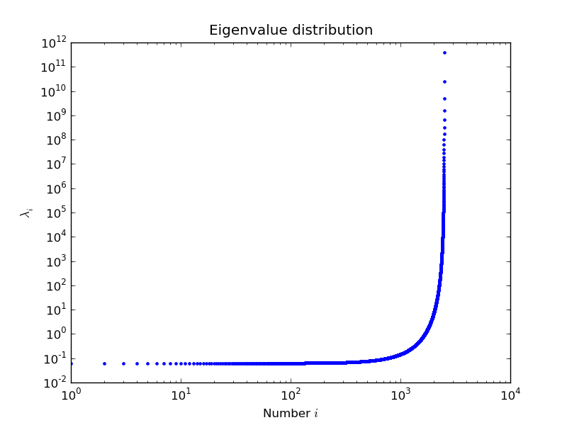
example by Nils Wagner:
output:
$ python examples/lobpcg_sakurai.py
Results by LOBPCG for n=2500

[ 0.06250083  0.06250028  0.06250007]

Exact eigenvalues

[ 0.06250005  0.0625002   0.06250044]

Elapsed time 7.01
