1.3.5. Some exercises

1.3.5.1. Array manipulations

1. Form the 2-D array (without typing it in explicitly):

   [[1,  6, 11],
    [2,  7, 12],
    [3,  8, 13],
    [4,  9, 14],
    [5, 10, 15]]
   

   and generate a new array containing its 2nd and 4th rows.

2. Divide each column of the array:

   >>> a = np.arange(25).reshape(5, 5)
   

   elementwise with the array b = np.array([1., 5, 10, 15, 20]). (Hint: np.newaxis).

3. Harder one: Generate a 10 x 3 array of random numbers (in range [0,1]). For each row, pick the number closest to 0.5.

   • Use abs and argsort to find the column j closest for each row.
   • Use fancy indexing to extract the numbers. (Hint: a[i,j] – the array i must contain the row numbers corresponding to stuff in j.)

1.3.5.2. Picture manipulation: Framing Lena

Let’s do some manipulations on numpy arrays by starting with the famous image of Lena (http://www.cs.cmu.edu/~chuck/lennapg/). scipy provides a 2D array of this image with the scipy.lena function:

>>> from scipy import misc
>>> lena = misc.lena()

Note: In older versions of scipy, you will find lena under scipy.lena()

Here are a few images we will be able to obtain with our manipulations: use different colormaps, crop the image, change some parts of the image.

• Let’s use the imshow function of pylab to display the image.

  In [3]: import pylab as plt
  In [4]: lena = misc.lena()
  In [5]: plt.imshow(lena)
  

• Lena is then displayed in false colors. A colormap must be

  specified for her to be displayed in grey.

  In [6]: plt.imshow(lena, cmap=plt.cm.gray)
  

• Create an array of the image with a narrower centering : for example,

  remove 30 pixels from all the borders of the image. To check the result, display this new array with imshow.

  In [9]: crop_lena = lena[30:-30,30:-30]
  

• We will now frame Lena’s face with a black locket. For this, we

  need to create a mask corresponding to the pixels we want to be black. The mask is defined by this condition (y-256)**2 + (x-256)**2

  In [15]: y, x = np.ogrid[0:512,0:512] # x and y indices of pixels
  In [16]: y.shape, x.shape
  Out[16]: ((512, 1), (1, 512))
  In [17]: centerx, centery = (256, 256) # center of the image
  In [18]: mask = ((y - centery)**2 + (x - centerx)**2) > 230**2 # circle
  

  then we assign the value 0 to the pixels of the image corresponding to the mask. The syntax is extremely simple and intuitive:

  In [19]: lena[mask] = 0
  In [20]: plt.imshow(lena)
  Out[20]: <matplotlib.image.AxesImage object at 0xa36534c>
  

• Follow-up: copy all instructions of this exercise in a script called

  lena_locket.py then execute this script in IPython with %run lena_locket.py.

  Change the circle to an ellipsoid.

1.3.5.3. Data statistics

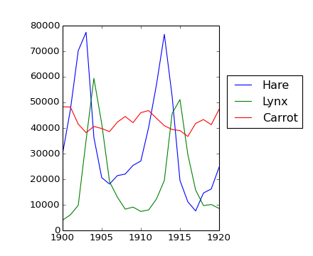
The data in populations.txt describes the populations of hares and lynxes (and carrots) in northern Canada during 20 years:

>>> data = np.loadtxt('data/populations.txt')
>>> year, hares, lynxes, carrots = data.T  # trick: columns to variables

>>> plt.axes([0.2, 0.1, 0.5, 0.8]) 
<matplotlib.axes.Axes object at ...>
>>> plt.plot(year, hares, year, lynxes, year, carrots) 
[<matplotlib.lines.Line2D object at ...>, ...]
>>> plt.legend(('Hare', 'Lynx', 'Carrot'), loc=(1.05, 0.5)) 
<matplotlib.legend.Legend object at ...>

[source code, hires.png, pdf]

Computes and print, based on the data in populations.txt...

1. The mean and std of the populations of each species for the years in the period.
2. Which year each species had the largest population.
3. Which species has the largest population for each year. (Hint: argsort & fancy indexing of np.array(['H', 'L', 'C']))
4. Which years any of the populations is above 50000. (Hint: comparisons and np.any)
5. The top 2 years for each species when they had the lowest populations. (Hint: argsort, fancy indexing)
6. Compare (plot) the change in hare population (see help(np.gradient)) and the number of lynxes. Check correlation (see help(np.corrcoef)).

... all without for-loops.

Solution: Python source file

1.3.5.4. Crude integral approximations

Write a function f(a, b, c) that returns . Form a 24x12x6 array containing its values in parameter ranges [0,1] x [0,1] x [0,1].

Approximate the 3-d integral

over this volume with the mean. The exact result is: — what is your relative error?

(Hints: use elementwise operations and broadcasting. You can make np.ogrid give a number of points in given range with np.ogrid[0:1:20j].)

Reminder Python functions:

def f(a, b, c):
    return some_result

Solution: Python source file

1.3.5.5. Mandelbrot set

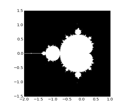
[source code, hires.png, pdf]

Write a script that computes the Mandelbrot fractal. The Mandelbrot iteration:

N_max = 50
some_threshold = 50

c = x + 1j*y

for j in xrange(N_max):
    z = z**2 + c

Point (x, y) belongs to the Mandelbrot set if < some_threshold.

Do this computation by:

1. Construct a grid of c = x + 1j*y values in range [-2, 1] x [-1.5, 1.5]
2. Do the iteration
3. Form the 2-d boolean mask indicating which points are in the set
4. Save the result to an image with:

>>> import matplotlib.pyplot as plt
>>> plt.imshow(mask.T, extent=[-2, 1, -1.5, 1.5]) 
<matplotlib.image.AxesImage object at ...>
>>> plt.gray()
>>> plt.savefig('mandelbrot.png')

Solution: Python source file

1.3.5.6. Markov chain

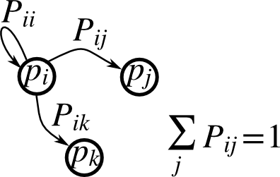
Markov chain transition matrix P, and probability distribution on the states p:

1. 0 <= P[i,j] <= 1: probability to go from state i to state j
2. Transition rule:
3. all(sum(P, axis=1) == 1), p.sum() == 1: normalization

Write a script that works with 5 states, and:

• Constructs a random matrix, and normalizes each row so that it is a transition matrix.
• Starts from a random (normalized) probability distribution p and takes 50 steps => p_50
• Computes the stationary distribution: the eigenvector of P.T with eigenvalue 1 (numerically: closest to 1) => p_stationary

Remember to normalize the eigenvector — I didn’t...

• Checks if p_50 and p_stationary are equal to tolerance 1e-5

Toolbox: np.random.rand, .dot(), np.linalg.eig, reductions, abs(), argmin, comparisons, all, np.linalg.norm, etc.

Solution: Python source file